ImpDAR plot_power() Tutorial

Introduction

This Notebook shows how, after picking a layer in ice or snow radar data, you would go about verifying that you have picked a single line (and not a combination of multiple lines, meaning you would have to repick that layer). But first, what does it mean to pick a layer? Picking is the process of digitizing reflectors within the glacier or ice sheet. As electromagnetic waves are sent through ice or snow, part of that wave is reflected back towards us and can be measured by a receiver antenna. How quickly that electromagnetic wave travels through a given medium is controlled by its permittivity. Each layer that you are seeing in a radargram is the result of permittivity contrasts between layers of different materials like ice, snow, firn, dust, and especially bedrock. Permittivity is heavily dependent on density and conductivity, and so you can clearly see the boundaries between ice-snow, ice-firn, and ice-bedrock where the permittivity changes..

While a pick’s power can vary along its length, just as a layer in ice or snow data can vary in depth depending on the surface and bed topography, power should not change drastically. It should be smooth during transitions if it changes at all. If you want to learn more about the way ImpDAR digitizes reflectors, please see the documentation about the imppick library here.

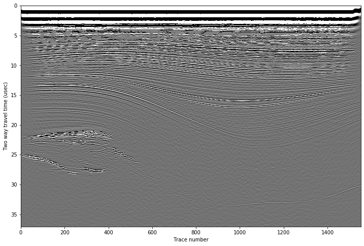
Let’s take a look at what a picked line looks like when you load it in ImpDAR. As an example, we will use a line collected in early 2020 from Hercules Dome, Antarctica which has already undergone the following processing steps: - the pretrigger data was cropped from the top of the data - a normal move-out correction was applied - the data was vertically bandpassed around a central frequency - then interpolated to regular grid spacing - migrated - and then picked

# We get annoying warnings about backends that are safe to ignore
import warnings
warnings.filterwarnings('ignore')

import numpy as np

%matplotlib inline
import matplotlib.pyplot as plt

import impdar
from impdar.lib import load
from impdar.lib import plot

Loading Data

#example matlab file name on disk
herc_mat_file = './data/HDGridE_x53_picks.mat'

#load the hercules dome data, now an ImpDAR RadarData object
dat = load.load('mat', herc_mat_file)[0]

#let's inspect our data file
plot.plot_radargram(dat)
plt.show()

#we can inspect the RadarData attributes here
vars(dat)

{'chan': 2,
 'data': array([[ 0.        ,  0.        ,  0.        , ...,  0.        ,
          0.        ,  0.        ],
        [ 0.        ,  0.        ,  0.        , ...,  0.        ,
          0.        ,  0.        ],
        [ 0.        ,  0.        ,  0.        , ...,  0.        ,
          0.        ,  0.        ],
        ...,
        [-0.79655623, -0.78011286, -0.70133412, ..., -0.60073161,
          0.28414989,  0.31941605],
        [-0.47651964, -0.47275442, -0.66581929, ..., -0.68916953,
          0.12462759,  0.28418875],
        [-0.21030229, -0.16901422, -0.61275566, ..., -0.746943  ,
         -0.04463077,  0.22238588]]),
 'decday': array([737454.07234843, 737454.07236893, 737454.07238942, ...,
        737454.10497516, 737454.1049937 , 737454.10501218]),
 'dt': 5e-09,
 'lat': array([-86.44000996, -86.43999383, -86.4399777 , ..., -86.41424587,
        -86.41422667, -86.41420724]),
 'long': array([252.85011635, 252.84942301, 252.84872966, ..., 251.78453531,
        251.78386739, 251.78320123]),
 'pressure': array([0, 0, 0, ..., 0, 0, 0], dtype=uint8),
 'snum': 7415,
 'tnum': 1553,
 'trace_int': array([0, 0, 0, ..., 0, 0, 0], dtype=uint8),
 'trace_num': array([   1,    2,    3, ..., 1551, 1552, 1553], dtype=uint16),
 'travel_time': array([0.0000e+00, 5.0000e-03, 1.0000e-02, ..., 3.7060e+01, 3.7065e+01,
        3.7070e+01]),
 'trig': 15,
 'trig_level': array([50, 50, 50, ..., 50, 50, 50], dtype=uint8),
 'nmo_depth': None,
 'elev': array([2595.40362135, 2595.41819483, 2595.43276831, ..., 2598.00668057,
        2597.93407972, 2597.87038998]),
 'dist': array([ 634.3,  639.3,  644.3, ..., 8384.3, 8389.3, 8394.3]),
 'x_coord': array([-369717.25869631, -369717.55360547, -369717.84851463, ...,
        -370193.10233268, -370193.66522139, -370194.2564618 ]),
 'y_coord': array([-114092.32989171, -114097.32118699, -114102.31248227, ...,
        -121824.02863999, -121828.9967592 , -121833.96162683]),
 'fn': '../data/HDGridE_x53_picks.mat',
 'data_dtype': dtype('<f8'),
 'flags': <impdar.lib.RadarFlags.RadarFlags at 0x7fb9a64862e8>,
 'picks': <impdar.lib.Picks.Picks at 0x7fb9a647bcf8>}

When we load the data file in ImpDAR, we can access the picks and their corresponding indices with dat.picks and dat.picks.picknums respectively. dat.picks.picknums returns an array back to you with indices that you can use when specifying which picked layer you would like to plot with the plot_power() method.

dat.picks.picknums

[1, 2]

We can also inspect dat.picks with the vars() method. Otherwise, you will only get back:

dat.picks

<impdar.lib.Picks.Picks at 0x7fb9a647bcf8>

vars(dat.picks)

{'samp1': array([[  nan,   nan,   nan, ...,   nan,   nan,   nan],
        [4892., 4892.,   nan, ..., 2711., 2709.,   nan]]),
 'samp2': array([[  nan,   nan,   nan, ...,   nan,   nan,   nan],
        [4925., 4925.,   nan, ..., 2731., 2728.,   nan]]),
 'samp3': array([[  nan,   nan,   nan, ...,   nan,   nan,   nan],
        [4941., 4944.,   nan, ..., 2749., 2746.,   nan]]),
 'time': array([[nan, nan, nan, ..., nan, nan, nan],
        [nan, nan, nan, ..., nan, nan, nan]]),
 'power': array([[        nan,         nan,         nan, ...,         nan,
                 nan,         nan],
        [22.82906175, 30.01928916,         nan, ..., 59.5785543 ,
         45.63542284,         nan]]),
 'picknums': [1, 2],
 'lasttrace': <impdar.lib.LastTrace.LastTrace at 0x7fb9cc33fb70>,
 'lt': <impdar.lib.LeaderTrailer.LeaderTrailer at 0x7fb9cc33fba8>,
 'pickparams': <impdar.lib.PickParameters.PickParameters at 0x7fb99785fcc0>,
 'radardata': <impdar.lib.RadarData.RadarData at 0x7fb9cc33fb38>,
 'lines': []}

Plotting Picks

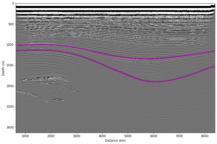
Now we are ready to plot the radargram along with the picks that we have previously saved. ImpDAR’s plot_radargram() method was designed for this purpose. Note, that without the optional parameters, plot_radargram() behaves exactly like the plot() method. However, now we can specify our x and y axis units as well as the colors that we would like to use to show our picked lines. Tthe default is magenta-green-magenta for the top, middle, and bottom of the wavelet used to pick lines, and this is what you will encounter in the GUI when you use the immpick command from the terminal.

plot.plot_radargram(dat, xdat='dist', ydat='depth', pick_colors='mgm')
plt.show()

Calculating Power Across Picks

Now we are ready to plot the power of our pick to verify it. We can call the plot_power() method from a Jupyter Notebook:

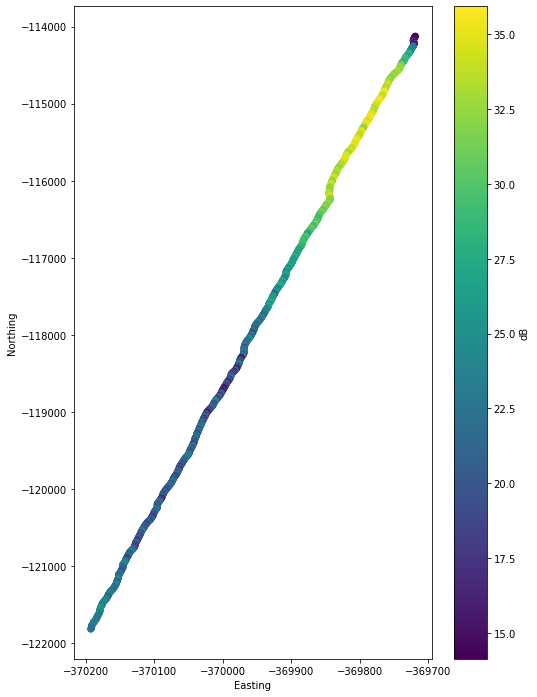
fig, ax = plot.plot_power(dat, 1)

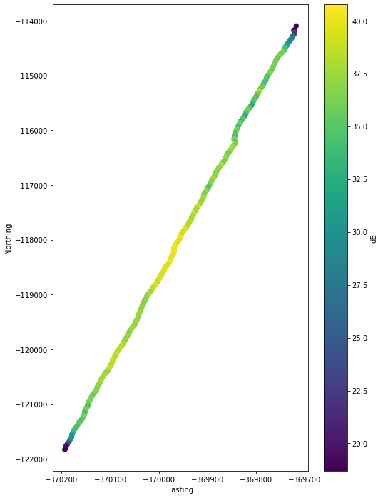
fig, ax = plot.plot_power(dat, 2)

If you wanted to run this method from the command line instead, you could use the following command to plot the power along the first pick:

impdar plot -power 1 HDGridE_x53_picks.mat

As you can see, our pick’s power does not change drastically along its length. This gives us more confidence that we have correctly identified a single layer within the snow or ice data. Doing this for each and every pick in a radargram profile would be a time-consuming process. But checking important layers at different depths in a radargram’s profile can help you quickly verify that you have isolated individual ice and snow layers.